This paper adds to existing evidence about the cost of increasing regulation in foregone economic growth and highlights the issue for policymakers. The effects of growing regulation on the pace of economic growth should be front and center in our economic policy discussions.

Our contribution presents economic growth estimates based on the largest available text-based regulation dataset. We find that regulatory growth has inhibited economic growth, which implies that Americans would likely see their incomes rise if the number of regulations were to fall. We illustrate the size of the effect by comparing an unconditional forecast in which regulations grow as expected with a conditional forecast in which the number of regulations is held constant.

Our results suggest that the increase in economic output from simply freezing regulation exceeds the effects from a simple extension of the Tax Cuts and Jobs Act (TCJA) that is currently being debated in Congress. Our estimates suggest that regulatory reform and deregulation should join tax reform as major policy issues in the 119th Congress.

Recent Economic Literature Highlights the Costs of Regulation

The discussion among academic economists of how regulations affect economic performance stretches at least as far back as Arthur Pigou and Nahid Aslanbeigui’s positive assessment of regulation in The Economics of Welfare (1938).REF However, more recent views have shifted to a more skeptical if not outright negative assessment of regulation’s economic effects. Daron Acemoglu, Simon Johnson, and James Robinson (2005) emphasize the effects on growth from differences in regulatory regimes as elements in larger institutional factors shaping growth.REF Antonio Ciccone and Elias Papaioannou (2007) reflect the earlier literature that focused on regulatory bureaucracy and its ill effects on firm formation and growth.REF

More recently, economists have produced quantitative estimates of how much regulations affect growth. W. Mark Crain and Nicole V. Crain (2014) developed economy-wide burden estimates that weighed down the U.S. economy by $2.4 trillion in 2012.REF Simeon Djankov, Caralee McLiesh, and Rita Maria Ramalho (2006) used a cross-country panel to estimate the effects of deregulation and found that countries in the quadrant containing the most regulated countries could increase their annual growth rates by 2.3 percentage points if they moved to the quadrant containing the least regulated countries.REF And Bentley Coffey, Patrick McLaughlin, and Pietro Peretto (2016) found that holding the level of regulations at their 1980 level would have resulted in an economy that was 25 percent larger in 2012, or about $4 trillion bigger in real gross domestic product (GDP) terms. Furthermore, that additional expansion equated to an increase in the annual growth rate of 0.8 percent per year.REF

Additionally, a number of studies emphasize the adverse effects of regulation on low-income households, largely through higher prices. For example, Dustin Chambers and Courtney Collins (2016) find that every 10 percent increase in total regulations leads to a 0.687 percent increase in the Consumer Price Index (CPI).REF Other studies have looked at the effects of regulatory delays, decreased investments, and regulatory barriers to entry.REF

How Would Freezing Regulation Affect the Economy?

Our work builds on this literature. We estimate the effects of regulation on economic output and prices using a medium-size Bayesian vector autoregression (BVAR). A BVAR is a set of interconnected equations that show how many economic variables tend to move together. Using Bayesian methods to estimate the model helps it to make more reliable predictions with limited data. BVARs are common tools for forecasting and policy analysis.REF

We use the model to produce an unconditional forecast and a forecast conditional on a path of regulatory restrictions that remains frozen at the end of the sample. We choose a forecast horizon of 10 years to match the 10-year budget window for Congress.

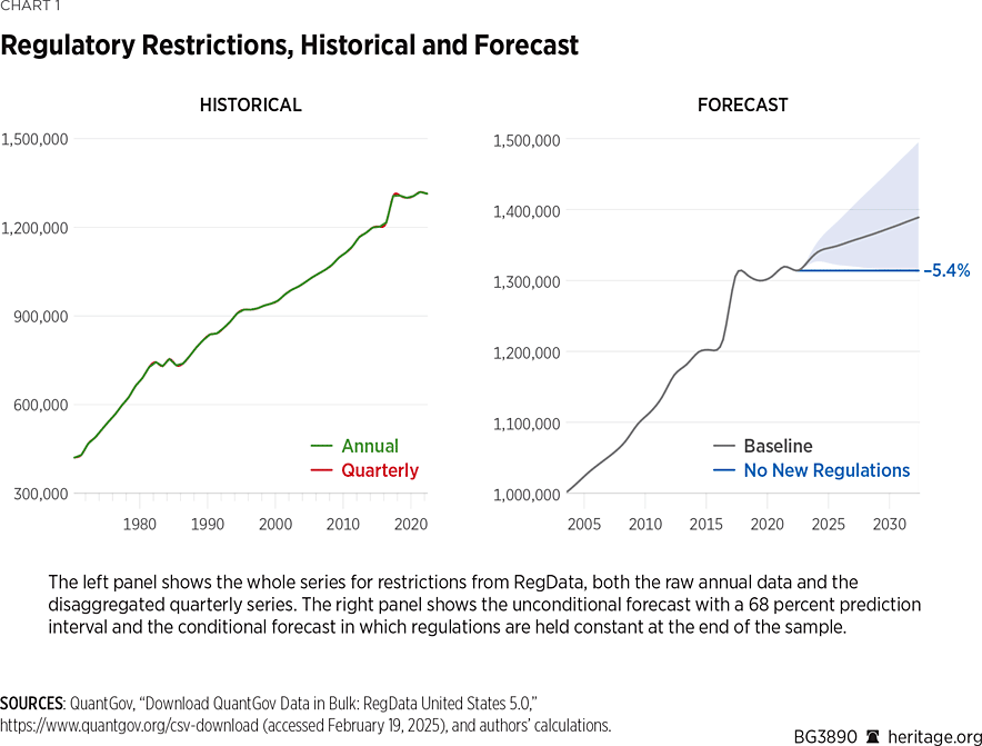
We use data on regulatory restrictions from RegData 5.0.REF This data source is a text-based database that processes the Federal Register and identifies five preselected words (“shall,” “must,” “may not,” “required,” and “prohibited”) that indicate restriction or compulsion. RegData then counts the incidence of these five different words. (The remaining variables are detailed in the appendix.)

Freezing regulations at the end of the sample reduces the forecast of regulations after 10 years by approximately 5.4 percent. The paths of the unconditional and conditional forecasts are shown in Chart 1. The line shows the median forecast, and the shaded area is the 68 percent prediction interval.

The left panel shows the whole series for restrictions from RegData, both the raw annual data and the disaggregated quarterly series. The right panel shows the unconditional forecast with a 68 percent prediction interval and the conditional forecast in which regulations are held constant at the end of the sample.

Freezing Regulations Grows the Economy While Reducing Inflation

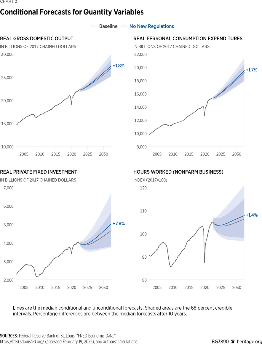
Freezing regulations produces a significant increase in the conditional forecast of the quantity variables after 10 years. These forecasts are shown in Chart 2. GDP goes up by 1.8 percent, consumption goes up by 1.7 percent, and hours worked goes up by 1.4 percent.

The primary channel for growth is through increased investment, which increases by 7.8 percent. Reducing the cost of complying with regulations raises the return to investment, so firms invest more. This result suggests that a combination of deregulatory actions directed at investment combined with tax policy changes that have the same goal could produce even greater gains in GDP than suggested by our current modelling.

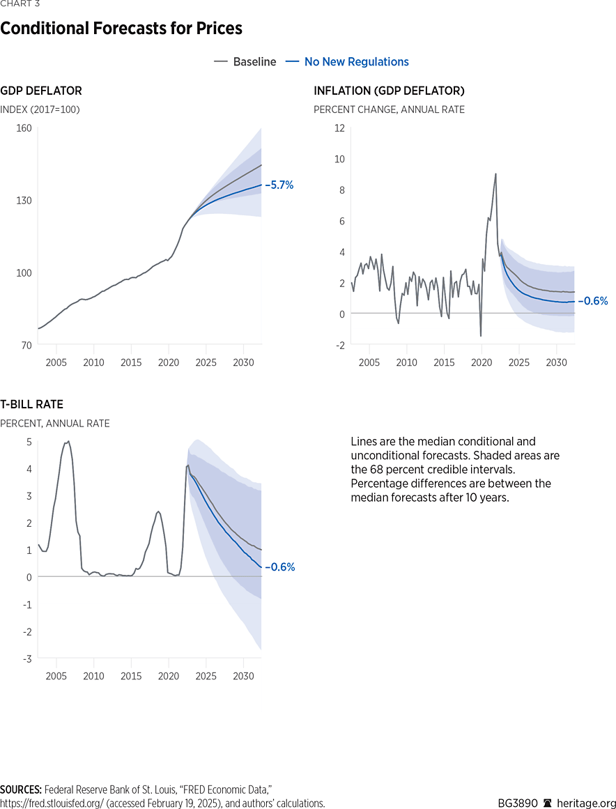
Moreover, freezing regulations is highly disinflationary. The GDP deflator falls 5.7 percent at the end of the 10-year forecast window. The path for the price level implies a reduction of the inflation rate by an average of 0.6 percent over the 10-year forecast window.

The reduction in inflation (as measured by the GDP deflator) gives space for Treasury rates to fall by 0.7 percent. Using the Congressional Budget Office (CBO) “rule of thumb” workbook, the combination of inflation and interest rate reductions would reduce the deficit by about $630 billion over 10 years.REF

Impulse Responses Show How Extra Regulations Affect the Economy

Many data analysts may be familiar with the equation for a line of best fit,

\[ y = \beta_0 + \beta_1 x \]

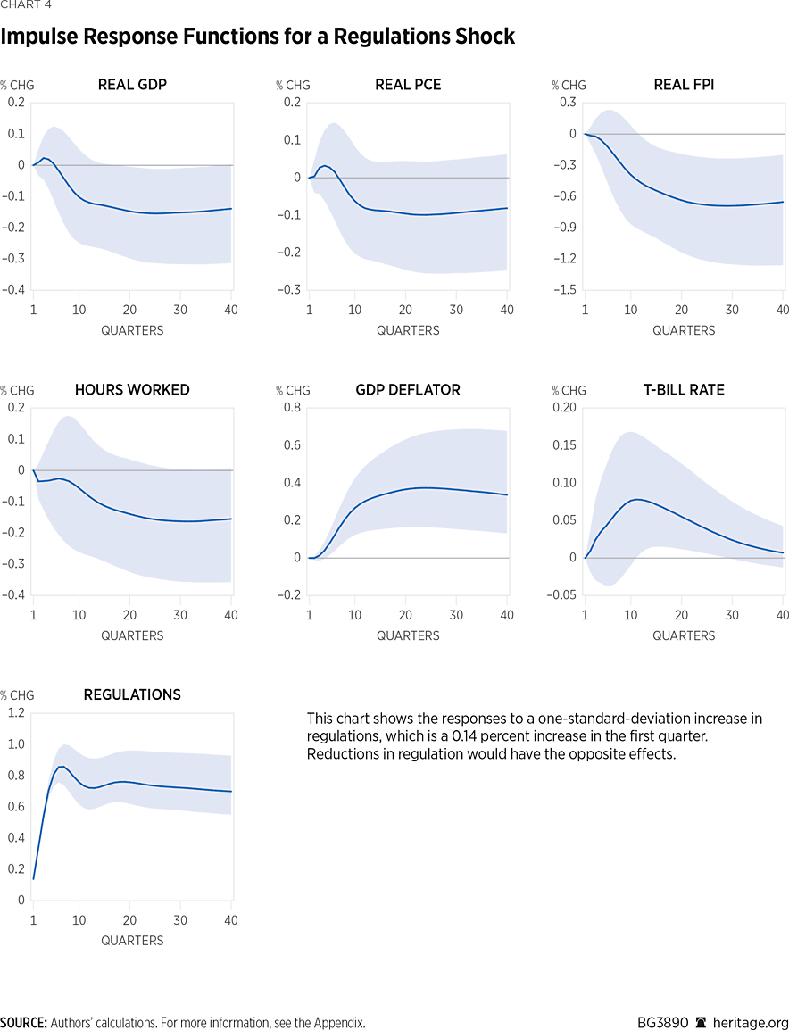
and its interpretation: A one-unit increase in x predicts a β₁-unit increase in y. A VAR has many equations and many inputs, so there are more coefficients describing the relationship between inputs and outputs. Instead, a common way to express the effects of unpredicted shocks is with impulse response functions. Impulse response functions show the predicted change in the data for several periods following an unexpected increase in one of the observations.

The impulse response functions for an average-size unexpected increase in regulations (about 0.14 percent) are shown in Chart 4. The solid line in the median response and the shaded area shows the uncertainty associated with the estimate.REF

An unexpected increase in regulations tends to reduce GDP, consumption, investment, and hours while increasing the price level and interest rates. Conversely, decreasing regulations would have the opposite effects. These effects take several quarters to reach their peak magnitude, but they are also long-lasting. Treasury rates return to baseline after about 10 years, and the other responses show about the same effect after 10 years as after five years.

Reducing Regulations Generates Additional Economic Growth Comparable to That Produced by Pro-Growth Tax Policy

Tax policy will be a major issue in the next Congress. We expect the 119th Congress to devote one of the two reconciliation bills to extending the Tax Cuts and Jobs Act of 2017 in addition to further reforming the tax code. Many provisions of the TCJA will expire at the end of 2025, raising the prospect of a tax increase on Americans. At the same time, rising federal debt and interest rates threaten to crowd out investment and slow economic growth.

Extending the TCJA would increase GDP by around 0.5 percent.REF The analysis presented in this study suggests that regulatory reform can offer additional economic growth as large as or larger than an item already at the top of the congressional agenda.

Congress has a tremendous opportunity to implement policy to foster economic growth for years to come. Regulatory reform should be one such policy that lawmakers pursue.

William W. Beach, DPhil, is a Visiting Fellow in the Center for Data Analysis at The Heritage Foundation. Parker Sheppard, PhD, is a Research Fellow in the Center for Data Analysis.

Appendix

The BVAR includes the following variables. Mnemonics from the Federal Reserve Economic Data (FRED) database are included in parentheses.

• Output: Real gross domestic product (GDPC1).
• Consumption: Real personal consumption expenditures (PCECC96).
• Investment: Real fixed private investment.

1. Fixed private investment (FPI).
2. Real private fixed investment chain-type price index (B007RG3Q086SBEA).

• Hours worked: Hours worked for all workers (HOANBS).
• Price level: GDP Deflator (GDPDEF).
• Interest rate: Treasury bill rate (TB3MS).
• Regulations: Total Regulatory Restrictions (RegData).

We collect the seven series into a vector and estimate the BVAR

\[y_t = a_0 + A_1 y_{t-1} + \dots + A_p y_{t-p} + \epsilon_t, \quad \text{with} \quad \epsilon_t \sim N(0, \Sigma)\]

where y_t is a 7 × 1 vector of data, a₀ is a 7 × 1 intercept, A_i are 7 × 7 coefficient matrices, and ε_t is a vector of normally distributed errors with variance-covariance matrix Σ.

We use a lag of three periods based on the Watanabe–Akaike Information Criterion (WAIC).REF Essentially, it measures how well each model fits the data with a penalty for using more parameters. Including a fourth lag raises WAIC because it does not increase accuracy enough to justify the additional parameters.

All data series are quarterly except for the regulatory restrictions. To avoid discarding the higher frequency in the other time series, we use the Chow-Lin methodREF as implemented in the R package tempdisagg.REF

The quarterly series for regulation counts is constructed by taking the first difference of the annual series. The Chow-Lin method regresses the annual first differences on a constant to produce a series of quarterly changes that add up to the respective annual changes. The initial value for regulatory count and the series of quarterly changes imply a corresponding quarterly series of counts.

We estimate the BVAR using the R package BVAR.REF The package implements the hierarchical method of Giannone, Lenza, and Primiceri (GLP) to estimate hyper-parameters for the prior distribution in the BVAR.REF GLP show that estimating hyper-parameters effectively balances the tightness of the prior to improve the model’s fit to data.

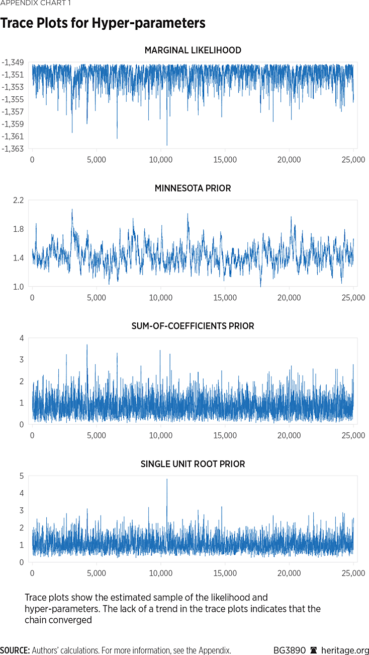
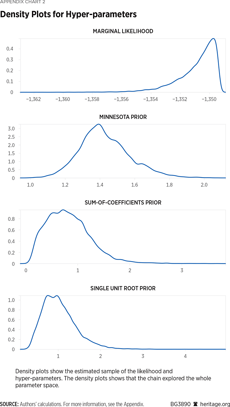
We draw one chain with 50,000 draws and discard the first 25,000 draws as a burn in. The acceptance rate was 0.336, in line with recommended targets that ensure the chain fully explores the parameter space. Geweke’s convergence diagnostic suggests that the chain in our sample has converged.REF Chart TK shows the trace and density plots for the marginal likelihood and the hyper-parameters from the Minnesota prior, the sum-of-coefficients-prior, and the single unit root prior.